It’s time to put all the pieces together and build a functional simulation. We’ll make use of the turtlebot3 software stack to get started. By the end of this post, we’ll have a robot autonomously navigating our world.
Introduction
In the spirit of accelerating the development of robotics applications with the use of ROS, there are various sets of packages available that can provide a working real or simulated robot. With well-defined interfaces between the different components of a typical ROS system, one can replace a component of that system with their own and get a complete platform upon which they can base their research.
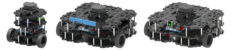
One such set of packages comes with turtlebot3. turtlebot3 is a differential-drive mobile robot aimed for educational, research, and prototyping purposes, and it’s available in the three variants shown above. The software stack of turtlebot3 allows us to operate either a real or a simulated robot. This means we don’t need to buy an actual robot to start experimenting with it.
If we dive deeper into the turtlebot3 software stack, we’ll find the ROS navigation stack at the heart of it. The ROS navigation stack is a generic navigation framework which can be used with any differential-drive robot and can also be extended to work with other types of robots. Similar stacks exist for the manipulation of robotic arms, and the control of drive bases, as well as robotic arms. It’s this modular nature of ROS that facilitates the development of robots. This is also why, even though last time we were only building up a gazebo world, this time, we can already have a robot autonomously navigating it. So let’s begin.
Preparation
We start by installing the necessary ROS packages. In case gazebo is not installed on your computer, follow the instructions in my Gazebo Simulation post. The commands below will fork the turtlebot3 packages in a grobot_ws workspace, install any dependencies in your computer, and build the workspace. Along with everything else, the grobot repository, which accompanies this post, will be placed in the workspace. It contains packages that will help us set up and run our examples.
> source /opt/ros/$ROS_DISTRO/setup.bash
> mkdir ~/grobot_ws
> cd ~/grobot_ws
> wstool init src https://github.com/nlamprian/grobot/raw/master/.grobot.rosinstall
> rosdep install --from-paths src --ignore-src --rosdistro=$ROS_DISTRO
> catkin build
> source devel/setup.bash
Do you remember how we said earlier that the navigation functionality is provided by the ROS navigation stack? Then what do the turtlebot3 packages offer? In essence, all they do is define a model for the robot, the configuration files for the navigation stack, and the launch files that get the system up and running. And just with those things alone, we can get a working robot in simulation. Pretty cool if you ask me. That’s not to say it’s easy to configure all this, but it’s nevertheless a good starting point.
Now, let’s focus on our own stack. The grobot repository contains the following packages:
grobot
├── grobot_bringup
├── grobot_gazebo
├── grobot_maps
└── grobot_utilities
grobot_gazebo holds all the gazebo resources (models, worlds, etc) and plugins we define, grobot_utilities contains auxiliary scripts, grobot_maps has the maps we generate, and grobot_bringup collects all the configuration and launch files for the tests we intend to run. In the next sections, we will go through how all these packages are built.
Setup of Gazebo Resources
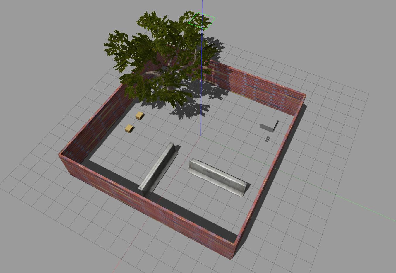
In the last post, we created a world in gazebo with models that we either borrowed from the online models repository, or created ourselves. Those models were placed in the default ~/.gazebo directory. This isn’t convenient if we want, for example, to launch the world on another computer. In that case, we’d have to make sure that we place the models in the ~/.gazebo directory before we can launch the simulation. Instead, this time we will store the models and the world in a ROS package, and configure the package such that gazebo can find the models in it. Let’s see how this is done.
We create a package grobot_gazebo, copy the world file into the worlds directory, and the models (only those we created ourselves, the others will be automatically downloaded) into the models directory.
grobot_gazebo
├── models
│   ├── box_z=0.5m/
│   └── building/
├── package.xml
└── worlds
    └── example.world
Next, we need to add gazebo_ros as a dependency to the package, and two exports in the package.xml.
  <depend>gazebo_ros</depend>
  <export>
    <gazebo_ros gazebo_media_path="${prefix}" />
    <gazebo_ros gazebo_model_path="${prefix}/models" />
  </export>
At this point, we can directly reference the world in a launch file, and when gazebo searches for the models, it will be able to find them inside the package.
<launch>
  <include file="$(find gazebo_ros)/launch/empty_world.launch">
    <arg name="world_name" value="$(find grobot_gazebo)/worlds/example.world" />
  </include>
</launch>
You can try loading the world by running
> roslaunch grobot_bringup world.launch
Spawning of the Turtlebot Model
We’ve configured the world, and now we need to put the turtlebot3 in it. The turtlebot3 comes with its own robot description that defines its links and joints, and configures its properties, sensors, and diff drive controller. We won’t focus right now on how this happens. Instead, we’ll just load the description to the parameter server as it is. Then, we can call a script that will read the description from the parameter server and give it to gazebo. Gazebo will take care of interpreting the description and spawning the model in the world. And just like that, we get a robot which we can control, and from which we can read sensor data. You can give it a try by running
> roslaunch grobot_bringup bringup.launch
This will launch gazebo, spawn the turtlebot3 model, and also open rviz.
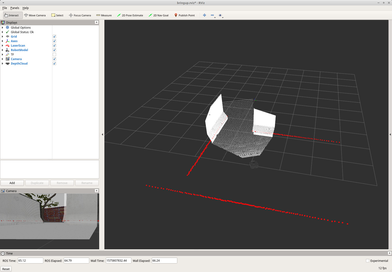
Doing a rostopic list will show us all the sensor topics published by gazebo, and the topic to which gazebo listens for velocity commands.
> rostopic list
/camera/depth/image_raw
/camera/depth/points
/camera/rgb/image_raw
/cmd_vel
/imu
/joint_states
/odom
/scan
...
As rviz is meant to visualize robot data, we aren’t able to see the actual world inside it. But we can get a view of the world from the sensor data. We can recognize object outlines from the laser scans (scan topic), object shapes from the point clouds (camera/depth/points topic), and the objects themselves from the camera images (camera/rgb/image_raw topic).
The cmd_vel topic is the interface for controlling the robot. This is where, later on, the navigation stack will publish to make the robot move. But we can also publish to the topic ourselves and move the robot manually. Run the following command and read the instructions in the terminal for teleoperating the robot with your keyboard
> roslaunch turtlebot3_teleop turtlebot3_teleop_key.launch
Map Generation
The next step is to generate a map. A robot uses a map for the purpose of localizing itself, as well as computing collision-free trajectories. A map constitutes a static representation of an environment. By comparing sensor data with the map, a robot is able to infer where it is, and thus how it needs to move in order to get to its destination. Also, by augmenting a map with live sensor data, we can eliminate the constraints of a static environment, and thus allow a robot to operate in a dynamic world.
One of the first and probably most well-known mapping packages that became available within ROS is gmapping. gmapping creates 2D occupancy grid maps based on laser scans. By keeping track of the pose of the robot, gmapping is able to accumulate laser scans and assemble them into a map. Even though gmapping is actively localizing the robot, errors manage to slip through and end up distorting the map. That’s why when the robot returns to a previously visited position, a loop closure could be detected that can provide a pose correction. This will be propagated backward and fix any errors that accumulated in the map during the process.
So, let’s use gmapping to create a map for our own world in gazebo. gmapping will be unaware that our robot runs in a simulation. All that gmapping does is listen to a topic for laser scans. It makes no difference whether these messages come from a real or simulated robot.
Run the following command to get the mapping process started.
> roslaunch grobot_bringup mapping.launch
This will launch the simulation (just as in the previous step), plus the gmapping node. Now, we just need to move the robot around, so we can collect enough laser scans to create a complete and accurate map. Just as before, we do this by teleoperating the robot with
> roslaunch turtlebot3_teleop turtlebot3_teleop_key.launch
We can see the map as it’s being built live in rviz. There, we can also observe the sudden changes in the map when the robot goes back to a known place, and gmapping attempts to fix the map. Once we are pleased with the result, we must save the map to a file, and then we are done.
> rosrun map_server map_saver -f `rospack find grobot_maps`/maps/example_world
As a final step, we need to go to grobot_maps/maps/example_world.yaml and change the image field. We remove the full path and leave only the filename.
Navigation
Finally, we reach the point where we make the robot autonomously navigate. We do this in four simple steps. Step one, launch the simulation. Step two, launch the map server with the example_world map. This is how, later on, move_base (the navigation planner) will retrieve the map. Step three, launch amcl. amcl implements a localization system.
Gazebo publishes odometry data (\(odom \leftarrow base\_footprint\)), which tells us where the robot is, given how the wheels have rotated. But this isn’t a reliable source of localization, since wheels can slip, their radius can change, and so on. This is where amcl comes in. It listens for laser scans and tries to localize the robot in the map (\(map \leftarrow odom\)). Combining these two sources of information, we get an estimation of the actual pose of the robot (\(map \leftarrow base\_footprint\)).
The robot is not localized when the simulation starts. To fix that, we have three options. We can start moving the robot, so amcl gets a good look at the environment (through the laser scans) until it manages to localize the robot correctly. Alternatively, we can use the 2D Pose Estimate feature in rviz, which is a manual process, so we move on to the third option. In our case, since it’s us that spawns the robot in the world, and we know exactly where the robot will appear, we can pass this information to amcl as an initial pose.
The final step is to launch move_base. move_base is what computes the trajectories for the robot. It works by generating a global path that is based on the map, and the robot tries to follow. It also continuously monitors the neighborhood of the robot such that the robot dynamically reacts to whatever is happening around it. move_base is already configured for turtlebot3, so we won’t focus on this here.
To give it a try, run
> roslaunch grobot_bringup navigation.launch
The robot is now waiting for a goal. In rviz, there is a 2D Nav Goal button. Press that button, then click somewhere in the viewer to select a point, drag to give a direction, and release. This will define a pose that will be sent to move_base, and soon the robot will start moving.
move_base receives a goal pose, computes a trajectory, and starts forwarding command velocities to gazebo. On the gazebo side, the diff drive controller of the robot consumes these velocities and computes the appropriate velocities for the wheels. And just like that, the puzzle is complete. Now go ahead, give a few navigation goals to the robot, and observe how it behaves.
Conclusion
So far, we’ve seen how to create, configure, and arrange any necessary resources, like models, worlds, and maps. We’ve also outlined the components of a robotic system that make a robot move. I hope I’ve clearly indicated how once you understood all the different pieces that go into creating a functional simulation, it’s not that hard to get something up and running. It might have taken me a year until I managed to create these gazebo posts, but it will only take you a few hours to get a robot autonomously navigating.
Next time, we will introduce a feedback loop into the mix. We will make the robot detect a visual marker and follow it as it moves in the world. In other words, we are going to configure a fully autonomous robot. We won’t be giving goals to the robot manually through rviz anymore, but we will have the robot look for its own targets and then try to reach them. In the mean time, we’ll explore some more interesting gazebo topics.